DEMOGRAPHY

Exercise 1

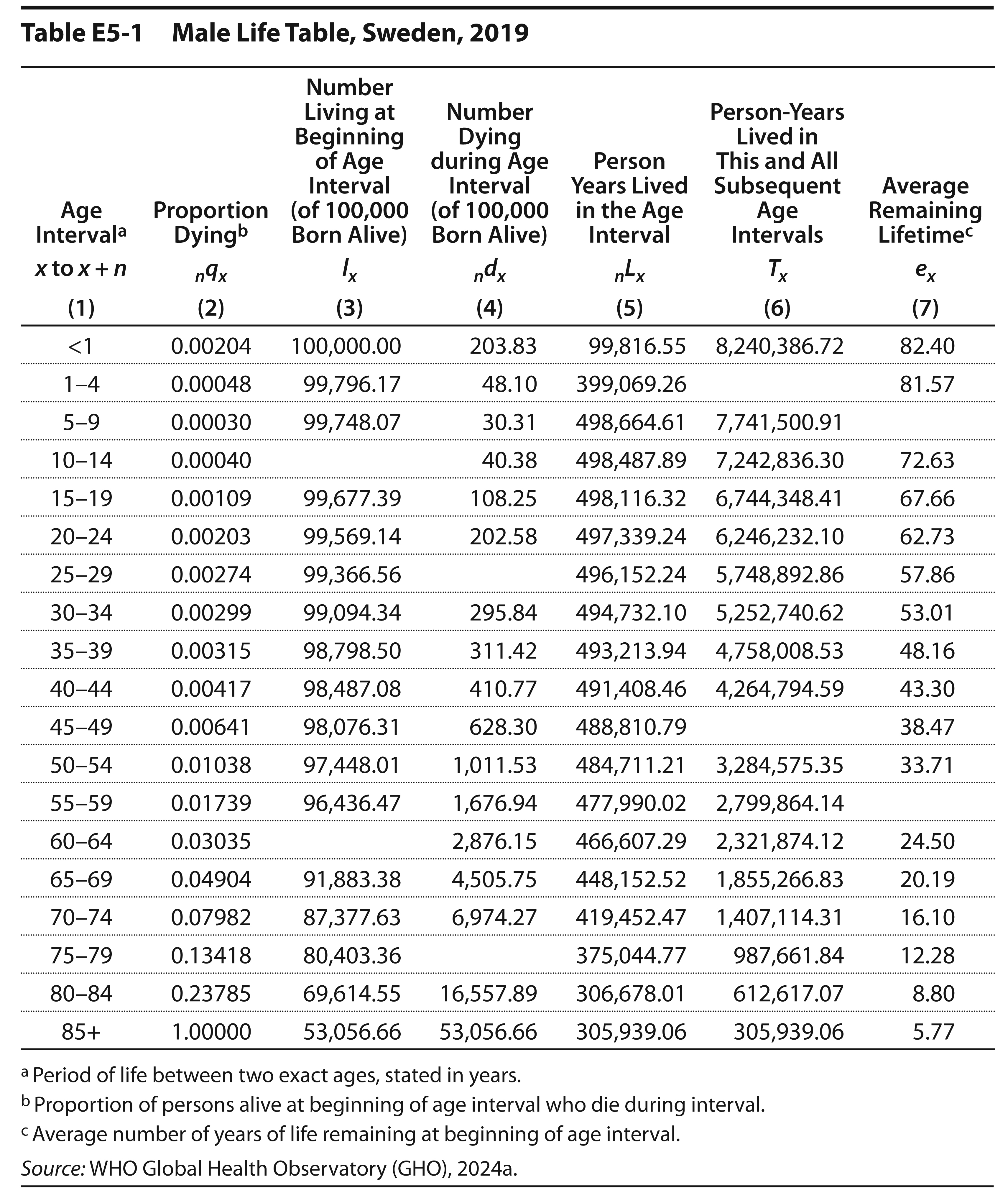
The following Table E5-1 is a male life table for Sweden according to the age-sex-specific death rates of 2019. Some blanks intentionally have been left in columns 3, 4, 6, and 7 of the table. Your task is to fill in those blanks, copying the computations used for determining the other entries for the same columns. What follows is an explanation of each of the columns, from left to right:

• Column 1 simply lists the age intervals. With three exceptions, we have used five-year intervals rather than single-year intervals; thus, this is an “abridged” life table. The exceptions are at either end of the age range. Infant mortality (age zero to one—a single year) is separated from early childhood mortality (age one to four—a 4-year interval). The terminal category (100 and over in this table) is open-ended.
• Column 2 (_nq_x) presents the assumed risk of dying over the n years beginning at age x for each of the age intervals. Each “mortality rate” is based on an age-sex-specific death rate. The rest of the table is generated from column 2.
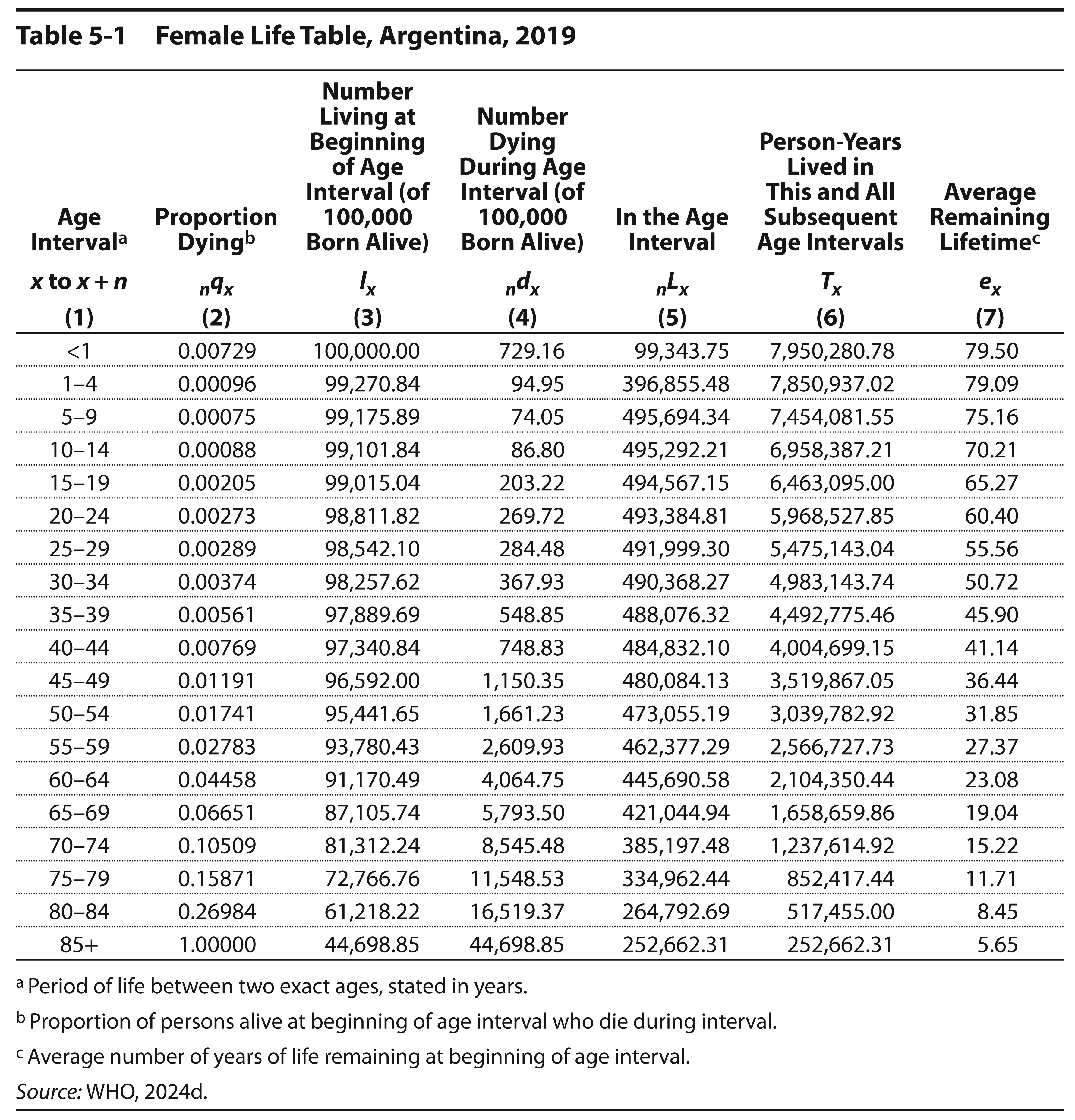
• Column 3 (l_x) and column 4 (_nd_x) are best explained together. We start at the top of column 3 with an arbitrary, large, hypothetical cohort (or “radix”); this table follows the convention of using 100,000 births. Then we trace what the fate of this hypothetical cohort would be if it experienced the probabilities of death listed in column 2. For instance, the 100,000 babies born experienced a probability of death of 0.00204 until their first birthday. This would result in 203.83 deaths by the first birthday. This is the entry for column 4 for the first age interval. How many boys would start their second year of life? We subtract the deaths (203.83) from those who started the first interval (100,000) and get 99,764.79, the next entry in column 3. Multiplying these 99,764.79 survivors by the probability of dying between the ages of one and four, or 0.00048, we find that 48.10 of them will die, the next entry in column 4, and so on, back and forth between columns 3 and 4. Algebraically stated:
  _nd_x = (_nq_x) × (l_x)

  and

  l_x+n = l_x − _nd_x

  where: x = exact age at the beginning of the age interval | n = number of years in the age interval

• Column 5 (_nL_x) is the number of person-years lived in the age interval by the survivors of the hypothetical cohort. In the first row, if there were 100,000 babies born and 99,788 survived the whole first year, how many person-years did they collectively live during that one-year age interval? It depends on when during the year death occurred. Because of the unusual pattern of death during infancy, demographers use a complex procedure to arrive at an estimate for the top entry in column 5. For subsequent age intervals, however, deaths are more evenly spread throughout the interval. Thus, for most of the age intervals beyond infancy, the entry will be very close to the average of (1) the number of people alive at the beginning of the interval and (2) the number alive at the end of the interval. You are not required to make such a complex interpolation here (note that the L is smaller than subsequent years in the first and second entries because it is a smaller age range of person years in the interval, age 0–1 in the first and ages 1–4 in the second, compared to 5-year ranges for all subsequent person years).
• Column 6 (T_x) is derived entirely from column 5 (_nL_x). It tells how many person-years will be lived by the survivors of the hypothetical cohort from any specified age until all are dead. Thus, the entry 8,240,386.72 at the top of column 6 indicates this hypothetical cohort collectively will have that many years of life among them before the last one dies. Arithmetically, the column is constructed by summing the number of years lived in each interval from the bottom row upward to the top in column 5. For example, the first T entry for column 6 equals the total of all L entries added together and then declines each interval from there. Stated algebraically:
  T_x =

  0 ∑ x=100+

  _nL_x
• Column 7 (e_x) tells the life expectancy remaining after each specified birthday. Take the top entry as an illustration, the life expectancy at birth (e₀). If there were 8,240,386.72 person-years of life to be shared among the 100,000 males who were born into the hypothetical cohort (see column 3), then there were 82.40 years per man. Algebraically stated:
  e_x =

  T_x l_x

  It can be thought of as the average number of years men in the hypothetical cohort would live, according to the death rates assumed in column 2. Life expectancies can be computed for later ages as well, and they frequently are. The exercise requests that you do so for ages five and fifty-five.